Dynamic Robot Model

See the Robotics_DynamicModel.project sample project in the installation directory of CODESYS under ..\CODESYS SoftMotion\Examples.

In order to limit the axis torques/forces during a movement, a dynamic model is required which calculates these values from the current axis state (position, velocity, and acceleration). This example includes the following parts:

Part 1 shows how to use an existing dynamic model in an application and the results of some sample movements.
Part 2 shows how to create a dynamic model for a SCARA robot based on an algorithm which is presented in the book "Modern Robotics" by K. M. Lynch and F. C. Park.

Structure of the application

Part 1: Using a dynamic model in an application

The code for this part is located in the TorqueLimitationDemofolder.
PLC_PRG is the main program, which includes a state machine that triggers test movements.
The movements can be monitored using the Trace.

Part 2: Creating a dynamic robot model

The code for the dynamic model is located in the DynModel folder.
DynModel_Scara2_Z is the dynamic model of the SCARA robot.
DynModel_Tests runs all tests of Test_DynModel_Scara2_Z to check for common mistakes.

The dynamic model is based on a SCARA robot with two revolute joints and one prismatic Z-axis. A figure of the robot with the required dimensions and coordinate systems for the dynamic model is shown below:

Dimension in Figure	Corresponding Variable Name in the Sample Project in the Function Block DynModel_Scara2_Z
`h0`	`baseHeight`
`h1`	`armOneHeight`
`h2`	`armTwoHeight`
`h3`	`zAxisLength`
`h4`	`zAxisOffset`
`l1`	`armOneLength`
`l1`	`armTwoLength`

Part 1: Using a dynamic model in an application

Using a dynamic model in an application requires a model which implements the ISMDynamics interface of the SM3_Dynamics library. The dynamic model from Part 2: Creating a dynamic robot model is used for this demonstration.

The model can be assigned to an axis group using SMC_GroupSetDynamics. This step requires setting up the gravitational acceleration with respect to the MCS. Because the SCARA in this example is mounted on the floor, the gravitational acceleration points in the positive z0 direction. The gravitational acceleration has to be specified in user units u/s². Because all lengths in this example have been defined in the user unit m, also the gravitational acceleration has to be specified in m/s².

SMC_ChangeDynamicLimits can be used to adjust the limits of each axis. Note that the axis group has to be enabled again using MC_GroupEnable in order to activate the new dynamic limits.

If additional masses are added to the TCP (for example, a tool or an object which is picked up by the robot), then SMC_GroupSetLoad can be used to define the load.

The PLC_PRG program contains all of the above components and executes two test movements:

Movement 1

Movement 2

Straight arm movement from (a0=0°, a1=0°, a2=0 m) to (a0=90°, a1=0°, a2=0,02 m):

Angled arm movement from (a0=0°, a1=-120°, a2=0 m) to (a0=90°, a1=-120°, a2=0,02 m):

Each movement is executed three consecutive times with the following boundary conditions:

The torque limit of all axes is infinite (unlimited).
The torque limit of Arm 2 is set to a lower value than the maximum reached torque during unlimited movement. The value was arbitrarily set to 2 Nm.
The torque limit of Arm 2 is still 2 Nm, and additionally a load has been applied at the TCP (mLoad=3 kg, lLoad=0.2 m):

The inertia calculation for the load has been simplified by using thin rods:

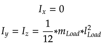The movements can be monitored in the trace. Movement 1 has the following results:

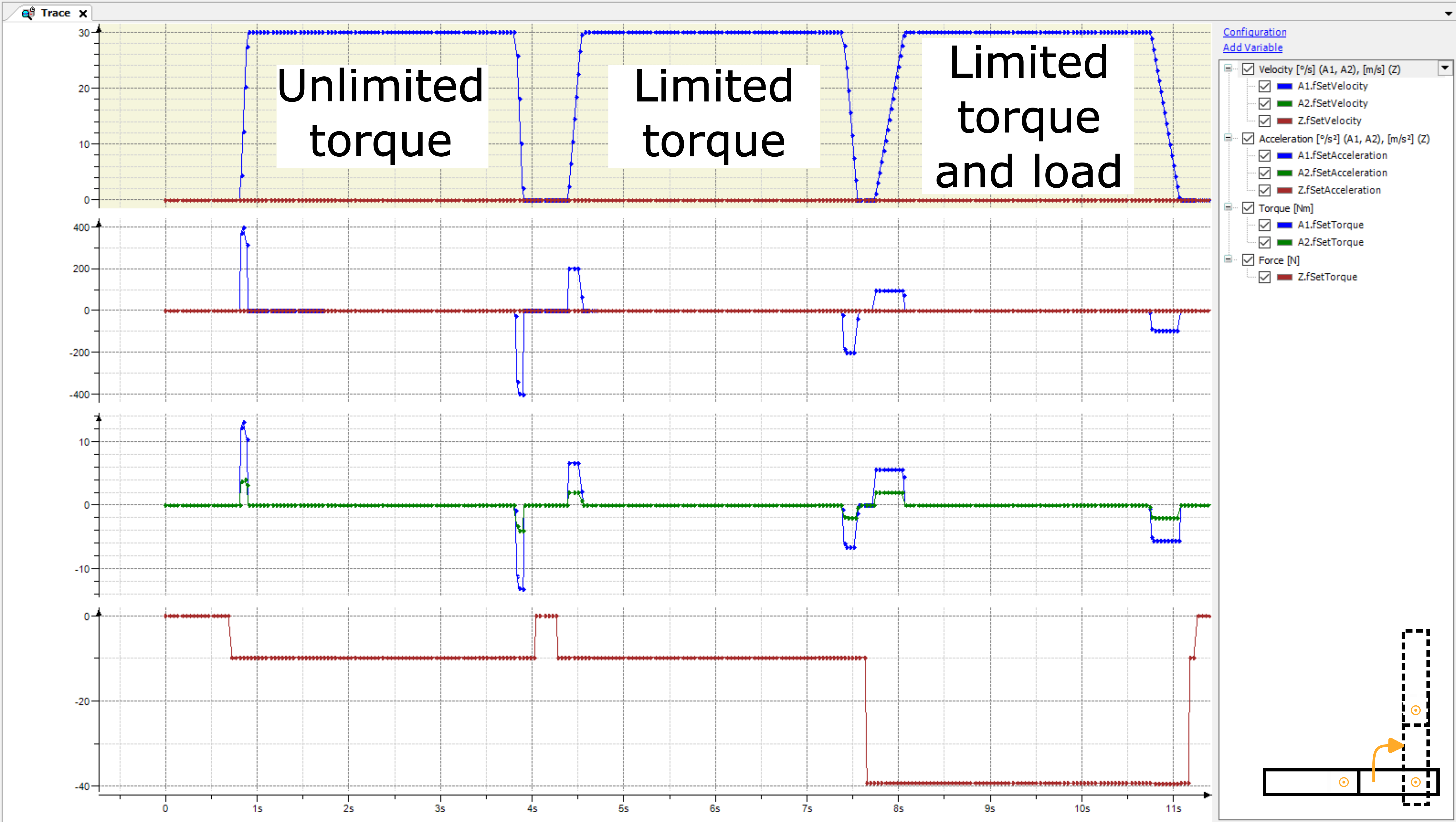
Even though Arm 2 does not move during Movement 1, the movement of Arm 1 results in a torque for Arm 2 during acceleration/deceleration. The calculated torque is sent to the drive and can potentially improve the controller loop in controller mode SMC_velocity or SMC_position. This is also called torque feed forward control.
The second pass with limited torque shows that the torque limit of Arm 2 leads to a slower movement of Arm 1. And that even if Arm 2 does not move. Without the dynamic model, the acceleration and deceleration of Arm 1 would have to be reduced manually for this movement in order to prevent excessive mechanical stress on Arm 2.
The third run with a load slows down the movement of Arm 1 even more in order to not violate the torque limit of Arm 2.

The advantages of using a dynamic model are obvious. To prevent excessive mechanical stress without dynamic model:

Either the dynamic limits for every movement would have to be set depending on the current state of the robot.
Or the dynamic limits of all axes would have to be decreased in such a way that all potential movements will not lead to excessive mechanical stress on any axis.

The first method is a complex task and it can be difficult to calculate reasonable limits, while the second method results in movements which are not as fast as possible most of the time. These drawbacks no longer exist with a dynamic model because the robot always moves as fast as possible while still respecting the mechanical limits of each axis.

These advantages are illustrated by the results of Movement 2:

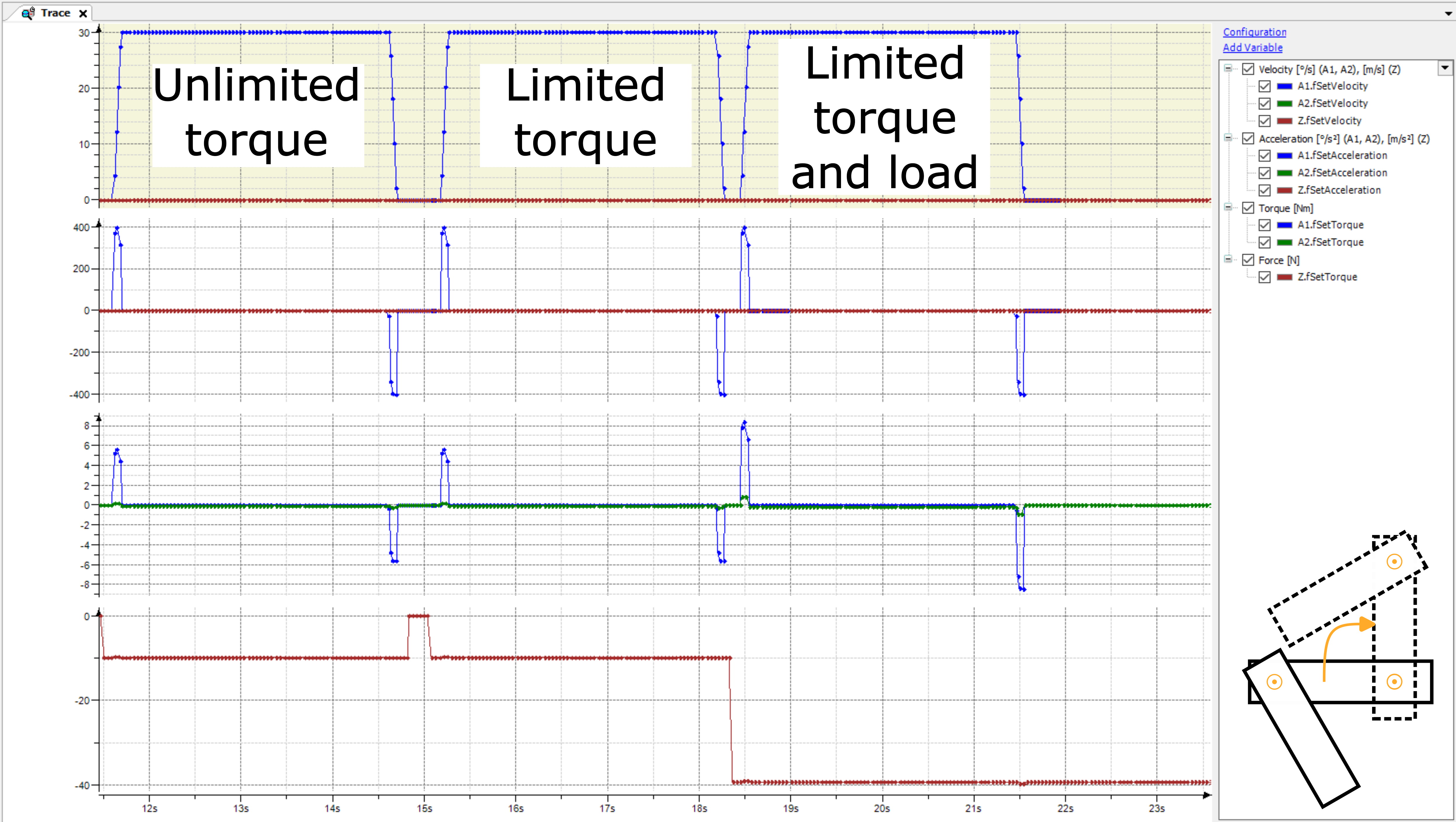
Due to the angled Arm 2, the resulting torque of Arm 2 is considerably lower than with Movement 1. Therefore, all three runs are never limited by the axis torque. If one had used adjusted dynamic limits based on Movement 1 (reduced acceleration and deceleration in order to not violate the torque limit of Arm 2), then this movement would have been slower than necessary.

Part 2: Creating a dynamic robot model

The model which is created in this example is based on an algorithm for open-chain robots as presented in the book "Modern Robotics" by K. M. Lynch and F. C. Park (see Chapter 8 "Dynamics of Open Chains"). The explanation of this algorithm is beyond the scope of this example. Instead, the example focuses on how to define the input values of the algorithm.

Simplifications

To make this example more understandable, some simplifications have been made:

The arm lengths l1 and l2 (distance between the axes of rotation) are used as their respective total arm length.
The center of mass is always located in the geometric center of each link.
The spatial inertia matrices of the arms and the Z-axis are calculated for thin rods.

Dynamic model requirements

In order to use the dynamic model in a SoftMotion application, this model has to implement the ISMDynamics interface of the SM3_Dynamics library.

The zero position, coordinate systems, and the positive direction of rotation of the dynamic model can theoretically deviate from the kinematic model. However, these differences have to be taken into consideration, and to simplify the dynamic model, it is therefore recommended to use the definitions of the kinematic model.

Because the dynamic model must compute torque values in Nm and forces in N, it has to convert the user unit u for lengths to SI units m. The conversion factor can be set by SMC_GroupSetUnits and is included in the addParams input of ISMDynamics.AxesStateToTorque. This example uses only m for lengths and can therefore ignore the conversion factor.

Specification of the geometric and dynamic data of the model

The IEC implementation of the algorithm presented in the book "Modern Robotics" by K. M. Lynch and F. C. Park (see Chapter 8 "Dynamics of Open Chains") requires the following input values:

The center of mass position of each link when the robot is in the home position. The position is specified in the coordinate system of the previous link (the first link is specified relative to the base coordinate system).
The spatial inertia matrix and mass of each link, expressed in the respective link frame.
The screw axis of each joint, expressed in the base frame.

Center of mass positions

The frames with the center of mass position of each link are as follows:

Link

Frame

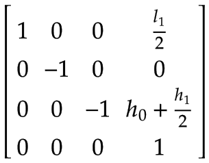
Arm 1

The center of mass of Arm 1, expressed in the base coordinate system x₀, y₀, z₀:

Note that there is a rotation of 180° around the x0-axis.

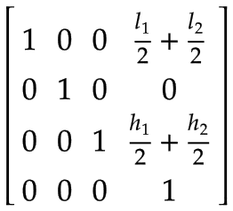
Arm 2

The center of mass of Arm 2, expressed in the coordinate system of Arm 1:

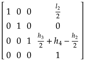
Z-axis

The center of mass of the Z-axis expressed in the coordinate system of Arm 2:

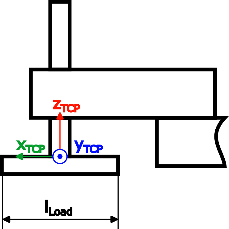
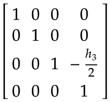
Tool Center Point (TCP)

One additional frame to handle an arbitrary load at the TCP (for example, by a tool, a product, or a combination of both), expressed in the coordinate system of the Z-axis:

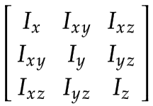
Spatial inertia matrices

The spatial inertia values have to be expressed in the respective link frame. Since the frames are defined at the center of mass, the spatial inertia can be represented by a 3x3 rotational inertia matrix and the mass of the body.

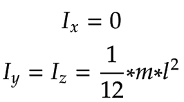
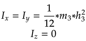
With the simplification of using thin rods for the joints, the components of the rotational inertia matrix are as follows:

Link

Components of the rotational inertia matrix

Arm 1, Arm 2

Arm 1 and Arm 2 with their corresponding mass m1 and m2, and length l1 and l2:

Z-axis

Screw axes

The screw axes of all joints have to be expressed relative to the base coordinate system x₀, y₀, z₀.

Link

Screw Axis

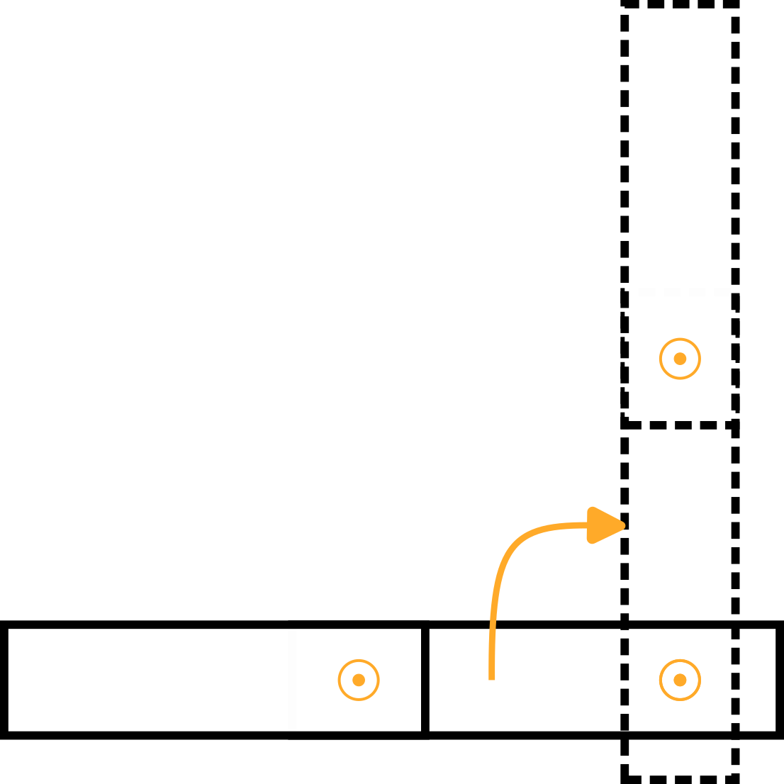
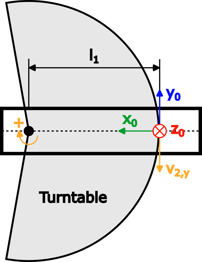
Arm 1

Imagine a turntable which rotates around Joint 1 in the positive direction with an angular velocity of 1 rad/s.

Expressed in the base coordinate system, this is a positive rotation around the z₀-axis according to the right-hand rule:

Because the axis of rotation of Arm 1 is equal to the center of the base coordinate system, the linear velocity is zero:

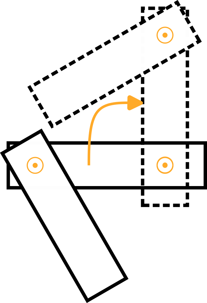
Arm 2

Imagine again a turntable which rotates around Joint 2 in the positive direction with an angular velocity of 1 rad/s. This case is displayed below as a top view of Arm 1:

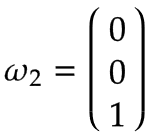
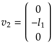
As for Arm 1, the angular velocity is:

The figure shows the resulting linear velocity v_2,y, which points in negative y₀ direction and is equal to v_2,y=-ω_2,z * l₁.

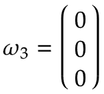
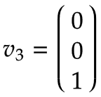
Z-axis

The Z-axis is a prismatic axis for which the following rules apply:

The angular velocity vector ω is zero.
The linear velocity vector is a unit vector in the direction of positive translation.

This leads to the following vectors, expressed in the base coordinate system x₀, y₀, z₀:

Tests

The dynamic model can now be tested because all model parameters are defined. This section includes some basic tests of the model.

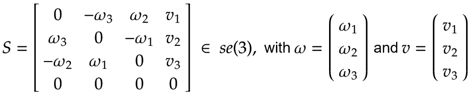
Checking the screw axes

A screw axis S with angular velocity ω and linear velocity v can be expressed as an element of se(3):

A forward transformation T can be executed with the screw axes S, an end effector frame M for the zero position of the robot, and the joint angle θ of each joint:

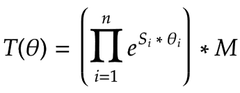The sample project already includes a function which solves this equation (see SMC_OpenChainKinematics_SolveForward). For more details, see the book "Modern Robotics" by K. M. Lynch and F. C. Park.

Using the forward transformation equation, one can now run a test with known axis positions and check if the transformation leads to the expected result.

Checking the torque calculation at standstill

To check the center of mass position frames, you can manually calculate the resulting axis torque in standstill for given axis positions and compare them to the computed values by the model. Because this example is based on a SCARA robot mounted on the floor, all axis positions in standstill will lead to the same torques or forces of the drives:

Joint	Resulting Torque/Force
Arm 1	Because Arm 1 is a revolute axis, the result is a torque: `M1=0 Nm`.
Arm 2	Because Arm 2 is a revolute axis, the result is a torque: `M2=0 Nm`.
Z-axis	Because the Z-axis is a prismatic axis, the result is a force: `F3=m3*g N` with gravitational acceleration `g`.